Computation of Thrust and Torque Coefficients Using Rotor Block

This example uses:

This example shows how the Rotor block in Aerospace Blockset™ can be used to compute the thrust and torque coefficients for an isolated rotor. This example compares the results of this computation with the values obtained using Blade Element Momentum Theory (BEMT) and where available, the experimental results from literature [1]. This example considers the variation of lift and drag coefficient with angle of attack, and the effect of profile drag in the BEMT computation. The results from the Rotor block are also compared with experimental results from literature.

In the BEMT computation, the fsolve (Optimization Toolbox) function in Optimization Toolbox™ is used to solve for the average inflow through the rotor disc.

Rotor model

The rotor model considered in this example is taken from [2]. These parameters are saved in Ref1Nb2Data.mat as the structure array rotorParams:

Nb: Number of blades in the rotor
R: Radius of the blade, in meters
e: Blade hinge-offset, in meters, measured from center of rotation
rc: Root cutout, in meters
c: Blade chord, in meters
rpm: Rotor revolutions per minute
a: blade section lift curve slope, in per rad

The root cutout is the inboard region of the blade where the rotor hub, hinges and the bearings are attached. This region has high drag coefficient and does not contribute to the lift.

Load the Ref1Nb2Data.mat file to add these parameters to the workspace:

refData = load('Ref1Nb2Data.mat');
Nb = refData.rotorParams.Nb; 
radius = refData.rotorParams.R; 
hingeOffset = refData.rotorParams.e; 
rootCutout = refData.rotorParams.rc; 
chord = refData.rotorParams.c; 
OmegaRPM = refData.rotorParams.rpm; 
Omega = convangvel(OmegaRPM, 'rpm' ,'rad/s'); 
sigma = Nb*chord/pi/radius; % rotor solidity
clalpha = refData.rotorParams.a;

Convert the reference rotor rotational velocity in RPM (Revolutions Per Minute) to rad/s using the convangvel function in Aerospace Toolbox. The rotor solidity $σ$ is the ratio of the blade area ( $N_{b} c R$ for constant chord blades) to the rotor disc area ( $π R^{2}$ ).

$σ = \frac{N_{b} c R}{π R^{2}} = \frac{N_{b} c}{π R}$

The lift and drag coefficient data [2] corresponding to the NACA0015 blade airfoil is saved in NACA0015Data.mat.

This file contains this date:

theta_NACA0015: Array of angle of attack values in degrees at which lift/drag coefficient data is available
CL_NACA0015: Array of lift coefficient values
CD_NACA0015: Array of drag coefficient values

Load the data in the NACA0015Data.mat file.

airfoilData = load('NACA0015data.mat');

Blade Element Momentum Theory (BEMT)

Blade Element Momentum Theory combines the Simple Momentum Theory (SMT) and the Blade Element Theory (BET) [1].

Simple Momentum Theory

In SMT, the rotor is an actuator disc that can support a pressure difference and accelerate the air through the disc. It is based on basic conservation laws of fluid mechanics.

Using this theory, the rotor thrust ( $T$ ) is related to the induced velocity ( $ν$ ) at the rotor disc by,

$T = 2 ρ A ν^{2}$

where $ρ$ is the density of air and $A$ is the rotor disc area ( $π R^{2}$ ).

Blade Element Theory

In BET, the blade is divided into airfoil sections capable of generating aerodynamic forces. This figure shows the blade section aerodynamics.

where,

$θ$ : pitch angle of blade
$ϕ$ : inflow angle
$α$ : aerodynamic angle of attack
$L$ : lift force at the blade section
$D$ : drag force at the blade section
$F_{z}$ : net force perpendicular to the disc plane
$F_{x}$ : net force tangential to the disc plane
$U_{P}$ : perpendicular air velocity seen by the blade
$U_{T}$ : tangential air velocity seen by the blade
$U$ : resultant velocity

and

$U = \sqrt{U_{T}^{2} + U_{P}^{2}}$

$ϕ = \tan^{- 1} \frac{U_{P}}{U_{T}}$

$α = θ - ϕ$ .

The sectional lift and drag forces are defined as

$L = \frac{1}{2} ρ U^{2} c c_{l}$

$D = \frac{1}{2} ρ U^{2} c c_{d}$ ,

where $ρ$ is the air density. $c_{l}$ and $c_{d}$ are the sectional lift and drag coefficients, and are typically functions of the angle of attack, Mach number and other parameters. In this example, we consider the coefficients to be functions of angle of attack alone (based on the available airfoil data).

The aerodynamic forces perpendicular and parallel to the disc plane are defined as

$F_{z} = L \cos ϕ - D \sin ϕ$

$F_{x} = L \sin ϕ + D \cos ϕ$

In hover, $U_{P} = ν$ , the induced velocity, and $U_{T} = Ω y$ , where $Ω$ is the rotational velocity of the rotor and $y$ is the dimensional radial location. The non-dimensional radial location is represented by $r = \frac{y}{R}$ .

Small angle approximations can be applied [1], to obtain

$U \approx U_{T} = Ω y, ϕ \approx \frac{U_{P}}{U_{T}} = \frac{ν}{Ω y} = \frac{λ}{r}$

$F_{z} = L, F_{x} = L ϕ + D$ .

Here, $λ = \frac{ν}{Ω R}$ is the non-dimensional induced velocity or inflow ratio.

The elemental thrust and torque can now be defined as

$Δ T = N_{b} F_{z} Δ r \approx N_{b} L Δ r$

$Δ Q = N_{b} F_{x} r R Δ r \approx N_{b} (L ϕ + D) r R Δ r$

Non-dimensionalizing the quantities to obtain the thrust and torque coefficients,

$Δ C_{T} = \frac{Δ T}{ρ π R^{2} (Ω R)^{2}} = \frac{N_{b} L Δ r}{ρ π R^{2} (Ω R)^{2}} = \frac{σ c_{l} r^{2}}{2} Δ r$

$Δ C_{Q} = \frac{Δ Q}{ρ π R^{3} (Ω R)^{2}} = \frac{N_{b} (L ϕ + D) r R Δ r}{ρ π R^{3} (Ω R)^{2}} = λ Δ C_{T} + \frac{σ c_{d} r^{3}}{2} Δ r$

Combining Momentum and Blade Element theories

Considering a rotor in hover, based on Momentum theory, the incremental thrust $Δ T$ for a rotor annulus of width $Δ y = R Δ r$ at radial position $r$ is

$Δ T = 2 ρ d A ν^{2} = 4 ρ π r R^{2} Δ r$ .

The corresponding non-dimensional thrust coefficient is

$Δ C_{T} = \frac{Δ T}{ρ π R^{2} (Ω R)^{2}} = 4 λ^{2} r Δ r$ .

To account for the blade tip-loss effects, the Prandtl tip loss function[2] $F$ can be is included as

$Δ C_{T} = 4 F λ^{2} r Δ r$

where $F = \frac{2}{π} e x p (- f), f = \frac{N_{b}}{2} \frac{1 - r}{r ϕ}$ .

Based on BET, the incremental thrust coefficient for the annulus is

$Δ C_{T} = \frac{σ c_{l}}{2} r^{2} Δ r$ .

The incremental torque coefficient $Δ C_{Q}$ is

$Δ C_{Q} = λ Δ C_{T} + \frac{σ c_{d}}{2} r^{3} Δ r$ .

Since the lift and drag coefficients depend on the local angle of attack, $α$ , using interpolation on the available reference data, the coefficient values can be obtained at the required $α$ .

The angle of attack is computed as

$α = θ - ϕ = θ - \frac{λ}{r}$ .

Here, $θ$ is the blade pitch angle at a radial location and depends on the blade twist and the pitch input. The reference blade considered in this example is untwisted and as pitch input, only the collective pitch( $θ_{0}$ ) variation is considered.

Hence you have

$θ = θ_{0}$ .

Considering the two equations for incremental thrust coefficient, you get

$4 F λ^{2} r Δ r = \frac{σ c_{l}}{2} r^{2} Δ r$ .

Solving the above equation at each radial location $r$ , the non-dimensional induced velocity ( $λ$ ) at the point can be computed. You can use this to compute the thrust and torque coefficients.

Rotor Block

The Rotor block in Aerospace Blockset can be used to compute the aerodynamic forces and moments in all three dimensions for an isolated rotor or propeller. This computation requires the mechanical parameters of the rotor including the thrust and torque coefficients as inputs. These coefficients can be obtained experimentally by doing a static thrust and torque analysis. This is the approach typically followed, especially in case of small propellers used in multirotor vehicles like quadrotors. In scenarios where the experimental study is not possible, or a comparison is to be made between the experimentally obtained values and theoretical values, the Rotor block can be used.

The Rotor block assumes:

Constant chord along the blade span
Constant lift curve slope
Profile drag contribution neglected
Only linear, or ideal twist distribution

Variation of Thrust and Torque Coefficients with Collective Pitch Input

Compute the values of $C_{T}$ and $C_{Q}$ corresponding to different values of collective pitch input $θ_{0}$ . Based on reference data, the range of collective pitch inputs considered here is from $0^{°}$ to $1 2^{°}$ .

theta0Array = 0:12;

The following matrices are used to save the thrust and torque coefficient results obtained using the two approaches. In case of BEMT computation, the torque coefficient values are computed with and without the inclusion of profile drag component. Save the values in the two columns of CQArrayBEMT.

CTArrayBEMT = zeros(length(theta0Array),1); 
CQArrayBEMT = zeros(length(theta0Array),2); 
CTArrayRotor = zeros(length(theta0Array),1); 
CQArrayRotor = zeros(length(theta0Array),1);

Computation Using BEMT

Compute net thrust and torque coefficients using BEMT by calculating the incremental values of the coefficients at each radial location and then summing up.

Nelements = 100; % number of radial elements
xnodes = linspace((rootCutout-hingeOffset)/(radius-hingeOffset),1,Nelements+1); % radial locations
delr = diff(xnodes); % corresponding to deltar in equations

Compute lift and drag coefficients, $c_{l}$ and $c_{d}$ at each radial location, using the function handles 'computeCl' and 'computeCd' with alpha ( $α$ ) as the input argument.

computeCl=@(alpha)interp1(airfoilData.theta_NACA0015, airfoilData.CL_NACA0015, convang(alpha,'rad','deg'));
computeCd=@(alpha)interp1(airfoilData.theta_NACA0015, airfoilData.CD_NACA0015, convang(alpha,'rad','deg'));

Compute the angle of attack $α$ at each radial location and convert to degrees using the convang function in Aerospace Toolbox. For interpolation, use interp1 function in MATLAB®.

To incorporate tip loss, use Prandtl's tip-loss function. Implement this as a function handle with the non-dimensional radial location $(r)$ and the inflow ( $λ$ ) as input arguments.

F = @(r,lambda)(2/pi)*acos(exp(-.5*Nb*((1-r)/(r*(lambda/r)))));

To solve for $λ$ at each radial location, use the fsolve (Optimization Toolbox) function in Optimization Toolbox. The default 'trust-region-dogleg' algorithm is used here to solving the equation. Set the initial guess for the fsolve function using the initInflow variable.

initInflow = 0.01; 
opts = optimset('Display','off');

Compute the net thrust and torque coefficients by looping over the range of collective pitch values, and the number of radial locations (for each pitch input).

Use the convang function to convert the collective pitch angle to radians. Compute the torque coefficient two ways, with and without the profile drag component.

for thetaInd = 1:length(theta0Array) % loop for collective pitch input
    theta0 = convang(theta0Array(thetaInd),'deg','rad');

    CT = 0; % initializing CT
    % initializing CQ
    CQwithDrag = 0; % with profile drag effect included
    CQwithoutDrag = 0; % without profile drag

    for rInd = 1:Nelements-1 % loop for radial locations
        r  =xnodes(rInd)+delr(rInd)/2;

        % solving for lambda at r
        lambdaVal = fsolve(@(lambda)4*F(r,lambda)*lambda^2*r-.5*sigma*r^2*(computeCl(theta0 - (lambda/r))),initInflow, opts);

        % computing incremental thrust coefficient
        dCT = 4*F(r,lambdaVal)*lambdaVal^2*r*delr(rInd);

        CT = CT + dCT;
        CQwithDrag = CQwithDrag + lambdaVal*dCT+ 0.5*sigma*computeCd(theta0 - (lambdaVal/r))*r^3*delr(rInd);
        CQwithoutDrag = CQwithoutDrag + lambdaVal*dCT;
    end
    CTArrayBEMT(thetaInd) = CT;
    CQArrayBEMT(thetaInd,1) = CQwithDrag;
    CQArrayBEMT(thetaInd,2) = CQwithoutDrag;
end

Computation Using Rotor block

To compute the thrust and torque coefficients using Rotor block in the Aerospace blockset, use the Simulink® model, CTCQcomputation.slx.

The Model Callbacks function adds the reference parameters to the model and the mask parameters R (radius), c (chord), e (hinge offset), clalpha (lift curve slope) are set to the reference values. The twist type is set to linear with the root pitch angle ( $θ_{0}$ ) set to the collective pitch angle (theta0). The input parameter to the block, density ( $ρ$ ) i set to the approximate sea-level value of $1.224$ $kg/m^3$, and rotor speed ( $Ω$ ) is set using the reference data (rpm).

To loop over the varying collective pitch angles, use a Simulink.SimulationInput object.

model = 'CTCQcomputation';
open_system(model);

simin(1:length(theta0Array)) = Simulink.SimulationInput(model);

for i = 1:length(theta0Array)
    theta0 = convang(theta0Array(i),'deg','rad');
    simin(i) = simin(i).setVariable('theta0',theta0);
end

simout = sim(simin,'ShowProgress','off');% turning off simulation progress messages

for i = 1:length(theta0Array)
    CTArrayRotor(i) = simout(1,i).CT;
    CQArrayRotor(i) = simout(1,i).CQ;
end

Analyzing Results

The experimental results for thrust and torque coefficients are obtained from [1] and saved in Ref1Nb2Data.mat. The experimental results present in the file are:

theta_data: collective pitch angles at which data is available
CTdata: thrust coefficient data
CQdata: torque coefficient data

Variation of thrust coefficient with collective pitch

Plot the variation of $C_{T}$ with $θ_{0}$ .

figure,plot(theta0Array,CTArrayBEMT,'b',...
    theta0Array, CTArrayRotor, 'r',refData.theta_data, refData.CTdata, 'k*')
ylim([0 0.01]);
xlabel('\theta_0')
ylabel('C_T')
ax = gca;
ax.YRuler.Exponent = 0; % setting y-axis ticks to standard notation
title('Variation of C_T with \theta_0')
legend('BEMT','Rotor Block', 'Experiment',...
    'Location','best','NumColumns',1,'FontSize',5);

Good correlation is observed between the experimental results, the results obtained using BEMT and the computed values obtained using Rotor block. Even though the computation using Rotor block assumes constant value for the lift coefficient, the effect of varying lift coefficient along the span (with angle of attack) is minimal.

Variation of torque coefficient with collective pitch

Plot the variation of $C_{Q}$ with $θ_{0}$ .

figure,plot(theta0Array,CQArrayBEMT(:,1),'b',...
    theta0Array,CQArrayBEMT(:,2),'--b',theta0Array,CQArrayRotor,'r',...
    refData.theta_data, refData.CQdata, 'k*')
xlabel('\theta_0')
ylabel('C_Q')
ylim([0 0.0006]);
title('Variation of C_Q with \theta_0')
ax = gca;
ax.YRuler.Exponent = 0;
legend('BEMT with profile drag', 'BEMT without profile drag','Rotor Block', 'Experiment',...
    'Location','best','NumColumns',1,'FontSize',5);

Good correlation is observed between the results obtained using BEMT, without profile drag, and the results obtained using Rotor block. Similarly, good correlation can be seen between the results obtained using BEMT, with profile drag, and the experimental results.

In the torque coefficient computation using Rotor block, it is assumed that the drag coefficient is small, and hence the profile drag contribution is neglected.

The following analysis studies the contribution of profile drag component in torque computation. For small values of $θ_{0}$ , the profile drag contribution over the entire rotor can be roughly approximated as

$\int_{0}^{1} \frac{σ c_{d}}{2} r^{3} d r = \frac{σ c_{d 0}}{8}$ .

Here, $c_{d 0}$ is considered as the mean drag coefficient.

Consider the approximate value of $c_{d 0}$ for NACA0015[2] in computing the profile drag component. Add the result to torque coefficient values obtained using Rotor block and compared with the BEMT values.

cd0 = 0.0113;
CQprofileApprox = sigma*cd0/8;
CQprofileRotor = CQArrayRotor+CQprofileApprox;
figure,plot(theta0Array,CQArrayBEMT(:,1),'b',theta0Array, CQprofileRotor,'r')
xlabel('\theta_0')
ylabel('C_Q')
ylim([0 0.0005]);
title('Variation of C_Q with \theta_0')
ax = gca;
ax.YRuler.Exponent = 0;
legend('BEMT with profile drag', 'Rotor Block with approximate profile drag',...
    'Location','best','NumColumns',1,'FontSize',5);

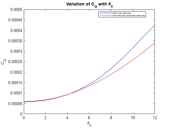
The analysis shows that for the specific rotor,

the approximation works well for smaller pitch input values, as would be the case in case of smaller rotors or propellers.
the effect of varying lift and drag coefficient values along the span on the computed torque coefficient is minimal.

Conclusion

The analysis shows that Rotor block can be used for the computation of thrust and torque coefficient values, with limitations.

Constant chord: In case of rotors with varying chord, computing the mean geometric chord[3] and using it in the computation is a reasonable approximation.
Constant lift coefficient: As shown in the above analysis, using the mean lift coefficient corresponding to the airfoil in the computation is a good approximation.
Low profile drag: The block neglects the effects of profile drag in the computation of torque coefficient.
Linear or ideal twist distribution: The block is enabled to consider linear or ideal twist variations along the span.

References

[1] Johnson W. (2013). Rotorcraft Aeromechanics. Cambridge University Press.

[2] Knight, M. and R. A. Hefner (1937). Static thrust analysis of the lifting airscrew. Technical Report 626, National Advisory Committee on Aeronautics.

[3] Leishman G.J. (2006). Principles of helicopter aerodynamics with CD extra. Cambridge University Press.