rvm

Rough volatility model (RVM)

Since R2023b

Description

Creates and displays an rvm object.

RVM (rough volatility model) objects are bivariate composite models, composed of two coupled and dissimilar univariate models that approximate continuous-time, rough stochastic volatility processes. The first univariate model is a geometric Brownian motion (GBM) model with a stochastic volatility function. This model usually corresponds to a price process whose variance rate is governed by the second univariate model. The second univariate model includes a Brownian semistationary process (BSS) without drift that describes the evolution of the variance rate that models the log volatility of the coupled GBM price process.

Creation

Syntax

RVM = rvm(Return,Volatility,Alpha,Beta)

RVM = rvm(___,Name=Value)

Description

example

RVM = rvm(Return,Volatility,Alpha,Beta) creates a default RVM object with Properties for these required arguments.

Specify the required input parameters as one of the following types:

A MATLAB^® array. Specifying an array indicates a static (non-time-varying) parametric specification. This array fully captures all implementation details, which are clearly associated with a parametric form.
A MATLAB function. Specifying a function provides indirect support for virtually any static, dynamic, linear, or nonlinear model. This parameter is supported via an interface because all implementation details are hidden and fully encapsulated by the function.

Note

You can specify combinations of array and function input parameters as needed.

Moreover, a parameter is identified as a deterministic function of time if the function accepts a scalar time t as its only input argument. Otherwise, a parameter is assumed to be a function of time t and state X(t) and is invoked with both input arguments.

example

RVM = rvm(___,Name=Value) creates an RVM object with additional options specified by one or more name-value arguments to set the Properties.

Input Arguments

expand all

`Return` — Expected (mean) instantaneous rate of return of GBM price process
scalar numeric | function_handle

Expected (mean) instantaneous of GBM price process, specified as an array, a numeric scalar, or a deterministic function of time as a function handle accepting time t or both time t and state X(t).

Data Types: double | function_handle

`Volatility` — Instantaneous volatility of BSS stochastic volatility process
scalar numeric | function_handle

Instantaneous volatility of the BSS stochastic volatility process, specified as an array, a numeric scalar, or a deterministic function of time as a function handle accepting time t. Volatility is also know as "volatility of volatility" or "volatility of variance" and is usually a nonnegative value.

Data Types: double | function_handle

`Alpha` — Kernel function parameter representing roughness index
scalar numeric

Kernel function parameter representing the roughness index, specified as numeric scalar. The value of Alpha should be in (-0.5, 0.5). The BSS process behaves locally like a fractional Brownian motion (fBm) with the Hurst index H = Alpha + 0.5.

Data Types: double

`Beta` — Kernel function parameter to control asymptotic memory properties
scalar numeric

Kernel function parameter to control asymptotic memory properties, specified as numeric scalar.

When you specify Beta > 0 for a gamma kernel specified using KernelType, if Alpha is in (-0.5, 0), the gamma kernel generates processes with short memory both for short and long time horizons.

When you specifyBeta > 0.5 for power-law kernel specified using KernelType, if you choose Alpha in (-0.5, 0) and Beta in (0.5, 1), the power-law kernel generates processes with short-memory property for small time scales and with long range memory for long time horizons.

Data Types: double

Name-Value Arguments

Specify optional pairs of arguments as Name1=Value1,...,NameN=ValueN, where Name is the argument name and Value is the corresponding value. Name-value arguments must appear after other arguments, but the order of the pairs does not matter.

Example: rvmObj = rvm(Return,Volatility,Alpha,Beta,KernelType="gamma")

`KernelType` — Type of kernel function assembling BSS process
`"gamma"` (default) | string with value `"gamma"` or `"power-law"` | character vector with value `'gamma'` or `'power-law'`

Type of kernel function (g(x)) assembling the kernel process, specified as a string or character vector for one of the following:

gamma — g(x) = x^ɑ * exp(-β * x)
power-law — g(x) = x^ɑ * (1+x)^{-β -
ɑ}

Data Types: string | char

`StartTime` — Starting time of first observation, applied to all state variables
`0` (default) | scalar

Starting time of the first observation, applied to all state variables, specified as a scalar.

Data Types: double

`StartState` — Initial values of state variables on all trials
`1` (default) | scalar, column vector, or matrix

Initial values of the state variables on all trials, specified as a scalar, column vector, or matrix.

If StartState is a scalar, rvm applies the same initial value to all state variables on all trials.

If StartState is a 2-by-1 column vector, rvm applies a unique initial value to each state variable on all trials.

If StartState is a 2-by-NTRIALS matrix, rvm applies a unique initial value to each state variable on each NTRIALS trials.

Data Types: double

`Correlation` — Correlation between Gaussian random variates drawn to generate bivariate Brownian motion vector (Wiener processes)
`2`-by-`2` identity matrix representing independent Gaussian processes (default) | numeric scalar | positive semidefinite matrix | deterministic function

Correlation between Gaussian random variates drawn to generate the bivariate Brownian motion vector (Wiener processes), specified as numeric scalar, a 2-by-2 positive semidefinite matrix, or a deterministic function C(t) that accepts the current time t and returns a 2-by-2 positive semidefinite correlation matrix. If Correlation is not a symmetric positive semidefinite matrix, use nearcorr to create a positive semidefinite matrix for a correlation matrix.

A Correlation matrix represents a static condition.

As a deterministic function of time, Correlation allows you to specify a dynamic correlation structure.

Data Types: double

`Simulation` — User-defined simulation function or SDE simulation method
simulation by Euler approximation (`simByEuler`) (default) | function | SDE simulation method

User-defined simulation function or SDE simulation method, specified as a function or SDE simulation method. The default is simByEuler.

Data Types: function_handle

Properties

expand all

`StartTime` — Starting time of first observation, applied to all state variables
`0` (default) | scalar

Starting time of first observation, applied to all state variables, returned as a scalar

Data Types: double

`StartState` — Initial values of state variables
`1` (default) | scalar, column vector, or matrix

Initial values of state variables, returned as a scalar, column vector, or matrix.

Data Types: double

`Correlation` — Correlation between Gaussian random variates drawn to generate Brownian motion vector (Wiener processes)
`2`-by-`2` identity matrix representing independent Gaussian processes (default) | positive semidefinite matrix

Correlation between Gaussian random variates drawn to generate the Brownian motion vector (Wiener processes), returned as a scalar or positive semidefinite matrix.

Data Types: double

`Return` — Expected (mean) instantaneous rate of return of GBM price process
scalar numeric | function_handle

Expected (mean) instantaneous rate of return of GBM price process, returned as a numeric scalar or function handle.

Data Types: double | function_handle

`Volatility` — Instantaneous volatility of BSS stochastic volatility process
scalar numeric | function_handle

Instantaneous volatility of the BSS stochastic volatility process, returned as a numeric scalar or function handle.

Data Types: double | function_handle

`Kernel` — Type of kernel process
string with value `"gamma"` or `"power-law"` | character vector with value `'gamma'` or `'power-law'`

Type of kernel process, returned as a string or character vector.

Data Types: string | char

`Alpha` — Kernel function parameter representing roughness index
scalar numeric

Kernel function parameter representing roughness index, returned as a numeric scalar.

Data Types: double

`Beta` — Kernel function parameter to control asymptotic memory properties
scalar numeric

Kernel function parameter to control asymptotic memory properties, returned as a numeric scalar.

Data Types: double

Object Functions

`simByEuler`	Simulate `RVM` or `roughbergomi` sample paths by Euler approximation
`simByHybrid`	Simulate `RVM` or `roughbergomi` sample paths by hybrid approximation

Examples

collapse all

Create `rvm` Object

Open Live Script

RVM (rough volatility model) objects are bivariate composite models, composed of two coupled and dissimilar univariate models that approximate continuous-time rough stochastic volatility processes.

Create an rvm object.

Return = 0.03;
Volatility = 0.2;
Alpha = 0.03;
Beta = 0.015;

rvmObj = rvm(Return,Volatility,Alpha,Beta,KernelType="gamma")

rvmObj = 
   Class RVM: Rough Stochastic Volatility
   ----------------------------------------
     Dimensions: State = 2, Brownian = 2
   ----------------------------------------
      StartTime: 0
     StartState: 1 (2x1 double array) 
    Correlation: 2x2 diagonal double array 
         Return: 0.03
     Volatility: 0.2
         Kernel: gamma
          Alpha: 0.03
           Beta: 0.015

More About

expand all

Instance Hierarchy

There are inheritance relationships among the SDE classes.

The following figure illustrates the inheritance relationships.

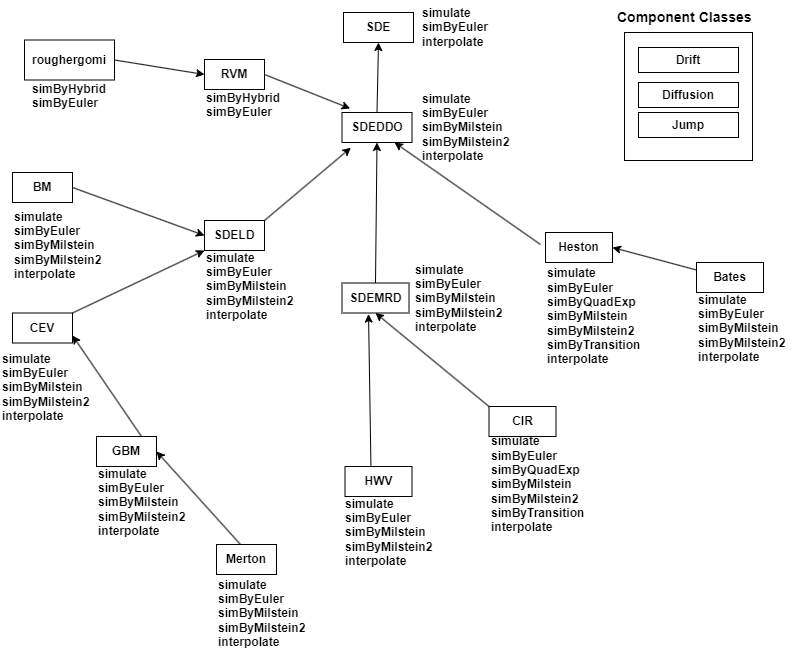
For more information, see SDE Class Hierarchy.

Algorithms

The rough volatility model (RVM) model allows you to simulate any vector-valued RVM of the form:

$\begin{array}{l} d X_{1 t} = B (t) X_{1 t} d t + X_{2 t} X_{1 t} d W_{1 t} \\ X_{2 t} = ξ e^{Y_{t}} \\ Y_{t} = \int_{- \infty}^{t} g (t - s) ν_{s} d W_{s} \end{array}$

The first equation is a geometric Brownian motion model with a stochastic volatility function.

The second equation is the process describing the evolution of the volatility rate of the coupled GBM process, where Y_t is a Brownian semistationary process.

g(t) is called a kernel function, which has the following properties:

For some $α \in (- \frac{1}{2}, \frac{1}{2}) \ {0}, x \in (0, 1)$ and L₀, there is a continuously differentiable, bounded away from zero, slowly varying function at zero: $g (x) = x^{α} L_{0} (x)$ , where ɑ = H -1/2 and H is a Hurst exponent.
The function g(x) is a continuously differentiable function with the derivative g' that is ultimately monotonic and satisfies $\int_{1}^{\infty} g^{'} {(x)}^{2} d x < \infty$ .
The kernel function is for some λ ≥ 0 and γ, such that γ > 1/2 when λ=0: $g (x) = e^{- λ x} x^{- γ} L_{1} (x)$ .

The Brownian semistationary process (Y_t in the general rough volatility model) is a two-sided Brownian motion (W) providing the fundamental noise innovations, with an amplitude that is modulated by a stochastic volatility process depending on W. This driving noise is then convolved with a deterministic kernel function g that specifies the dependence structure of Y_t. The process Y_t is also viewed as a moving average of volatility modulated Brownian noise. When you set the volatility of volatility = 1, the stationary Brownian moving averages are nested in this class of processes.

References

[1] Barndorff-Nielsen, O.E. and Schmiegel, J. “Brownian Semistationary Processes and Volatility / Intermittency.” Advanced Financial Modeling, Walter de Gruyter, Germany, 2009, pp. 1–26.

Version History

Introduced in R2023b

rvm

Description

Creation

Syntax

Description

Input Arguments

`Return` — Expected (mean) instantaneous rate of return of GBM price process
scalar numeric | function_handle

`Volatility` — Instantaneous volatility of BSS stochastic volatility process
scalar numeric | function_handle

`Alpha` — Kernel function parameter representing roughness index
scalar numeric

`Beta` — Kernel function parameter to control asymptotic memory properties
scalar numeric

`KernelType` — Type of kernel function assembling BSS process
`"gamma"` (default) | string with value `"gamma"` or `"power-law"` | character vector with value `'gamma'` or `'power-law'`

`StartTime` — Starting time of first observation, applied to all state variables
`0` (default) | scalar

`StartState` — Initial values of state variables on all trials
`1` (default) | scalar, column vector, or matrix

`Correlation` — Correlation between Gaussian random variates drawn to generate bivariate Brownian motion vector (Wiener processes)
`2`-by-`2` identity matrix representing independent Gaussian processes (default) | numeric scalar | positive semidefinite matrix | deterministic function

`Simulation` — User-defined simulation function or SDE simulation method
simulation by Euler approximation (`simByEuler`) (default) | function | SDE simulation method

Properties

`StartTime` — Starting time of first observation, applied to all state variables
`0` (default) | scalar

`StartState` — Initial values of state variables
`1` (default) | scalar, column vector, or matrix

`Correlation` — Correlation between Gaussian random variates drawn to generate Brownian motion vector (Wiener processes)
`2`-by-`2` identity matrix representing independent Gaussian processes (default) | positive semidefinite matrix

`Return` — Expected (mean) instantaneous rate of return of GBM price process
scalar numeric | function_handle

`Volatility` — Instantaneous volatility of BSS stochastic volatility process
scalar numeric | function_handle

`Kernel` — Type of kernel process
string with value `"gamma"` or `"power-law"` | character vector with value `'gamma'` or `'power-law'`

`Alpha` — Kernel function parameter representing roughness index
scalar numeric

`Beta` — Kernel function parameter to control asymptotic memory properties
scalar numeric

Object Functions

Examples

Create `rvm` Object

More About

Instance Hierarchy

Algorithms

References

Version History

See Also

Topics

rvm

Description

Creation

Syntax

Description

Input Arguments

Return — Expected (mean) instantaneous rate of return of GBM price process scalar numeric | function_handle

Volatility — Instantaneous volatility of BSS stochastic volatility process scalar numeric | function_handle

Alpha — Kernel function parameter representing roughness index scalar numeric

Beta — Kernel function parameter to control asymptotic memory properties scalar numeric

KernelType — Type of kernel function assembling BSS process "gamma" (default) | string with value "gamma" or "power-law" | character vector with value 'gamma' or 'power-law'

StartTime — Starting time of first observation, applied to all state variables 0 (default) | scalar

StartState — Initial values of state variables on all trials 1 (default) | scalar, column vector, or matrix

Correlation — Correlation between Gaussian random variates drawn to generate bivariate Brownian motion vector (Wiener processes) 2-by-2 identity matrix representing independent Gaussian processes (default) | numeric scalar | positive semidefinite matrix | deterministic function

Simulation — User-defined simulation function or SDE simulation method simulation by Euler approximation (simByEuler) (default) | function | SDE simulation method

Properties

StartTime — Starting time of first observation, applied to all state variables 0 (default) | scalar

StartState — Initial values of state variables 1 (default) | scalar, column vector, or matrix

Correlation — Correlation between Gaussian random variates drawn to generate Brownian motion vector (Wiener processes) 2-by-2 identity matrix representing independent Gaussian processes (default) | positive semidefinite matrix

Return — Expected (mean) instantaneous rate of return of GBM price process scalar numeric | function_handle

Volatility — Instantaneous volatility of BSS stochastic volatility process scalar numeric | function_handle

Kernel — Type of kernel process string with value "gamma" or "power-law" | character vector with value 'gamma' or 'power-law'

Alpha — Kernel function parameter representing roughness index scalar numeric

Beta — Kernel function parameter to control asymptotic memory properties scalar numeric

Object Functions

Examples

Create rvm Object

More About

Instance Hierarchy

Algorithms

References

Version History

See Also

Topics

`Return` — Expected (mean) instantaneous rate of return of GBM price process
scalar numeric | function_handle

`Volatility` — Instantaneous volatility of BSS stochastic volatility process
scalar numeric | function_handle

`Alpha` — Kernel function parameter representing roughness index
scalar numeric

`Beta` — Kernel function parameter to control asymptotic memory properties
scalar numeric

`KernelType` — Type of kernel function assembling BSS process
`"gamma"` (default) | string with value `"gamma"` or `"power-law"` | character vector with value `'gamma'` or `'power-law'`

`StartTime` — Starting time of first observation, applied to all state variables
`0` (default) | scalar

`StartState` — Initial values of state variables on all trials
`1` (default) | scalar, column vector, or matrix

`Correlation` — Correlation between Gaussian random variates drawn to generate bivariate Brownian motion vector (Wiener processes)
`2`-by-`2` identity matrix representing independent Gaussian processes (default) | numeric scalar | positive semidefinite matrix | deterministic function

`Simulation` — User-defined simulation function or SDE simulation method
simulation by Euler approximation (`simByEuler`) (default) | function | SDE simulation method

`StartTime` — Starting time of first observation, applied to all state variables
`0` (default) | scalar

`StartState` — Initial values of state variables
`1` (default) | scalar, column vector, or matrix

`Correlation` — Correlation between Gaussian random variates drawn to generate Brownian motion vector (Wiener processes)
`2`-by-`2` identity matrix representing independent Gaussian processes (default) | positive semidefinite matrix

`Return` — Expected (mean) instantaneous rate of return of GBM price process
scalar numeric | function_handle

`Volatility` — Instantaneous volatility of BSS stochastic volatility process
scalar numeric | function_handle

`Kernel` — Type of kernel process
string with value `"gamma"` or `"power-law"` | character vector with value `'gamma'` or `'power-law'`

`Alpha` — Kernel function parameter representing roughness index
scalar numeric

`Beta` — Kernel function parameter to control asymptotic memory properties
scalar numeric

Create `rvm` Object